Sentence Classification using CNN

ABSTRACT

Convolution Neural Networks are typically used in computer vision problems like image classification. Most of the computer vision systems todays at its core are based on CNNs from photo tagging to self driving cars. However we are going to look at the application of CNNs in NLP(Natural Language Processing).

BACKGROUND

Natural Language Processing

• Natural language is designed to make human communication efficient. As a result,
  • We omit a lot of “common sense” knowledge, which we assume the hearer/reader possesses.
  • We keep a lot of ambiguities, which we assume the hearer/reader knows how to resolve.
• This makes EVERY step in NLP hard.
  • Ambiguity is a “killer”!
  • Common sense reasoning is pre-required.

Word Embedding(or Word Vectors)

• Discrete representation- The vast majority of statistical NLP work regards, words as atomic symbols: hotel, conference, motel . In vector space terms, this is a vector with one 1 and everything else is zeroes. Every word is orthogonal to one another like $𝑤_{ℎ𝑜𝑡𝑒𝑙} \cdot 𝑤_{𝑚𝑜𝑡𝑒𝑙} =0$. Hence word similarity is not captured. Representing words as atomic symbols, leads to data sparsity, and usually means that we may need more data in order to successfully train statistical models.
• Continuous representation- We can embed words in $𝑅^𝐷$ with $D \leq V$ such that semantically close words are likewise `close’ in $𝑅^𝐷$. It will capture distributional similarity. One of the most successful ideas of modern statistical NLP.
  • Count Based Models- To make neighbors represent words, it uses count based co-occurrence matrix $\in 𝑅^{𝑉 × 𝑉}$. For example: LSA, LDA etc. It can be embed into $\in 𝑅^{𝐷×𝑉)}$ using SVD. Computational cost for SVD scales quadratically for $D×𝑉$ matrix: $O(𝐷𝑉^2)$ flops. Bad for millions of words or documents. Hard to incorporate new words or documents.
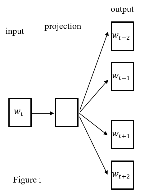
• Direct prediction Models– Here the idea is directly learning lower vector representation. For example: Feed forward neural language model, recurrent neural language model, Log-Linear language model(Continuous bag of words model, Continuous skip gram model). One of the most popular one is word2vec which based on Log-Linear language model. Word2vec instead of capturing co-occurrence counts directly, it predicts surrounding words of every word Fig.1 @fig:SentClassificationFigure1. Word2vec representation is pretty good in capturing syntactic and semantic relationship between words like: $𝑤_{𝑏𝑖𝑔}−𝑤_{𝑏𝑖𝑔𝑔𝑒𝑟} \approx 𝑤_{𝑠𝑙𝑜𝑤}−𝑤_{𝑠𝑙𝑜𝑤𝑒𝑟}$, $𝑤_{𝑓𝑟𝑎𝑛𝑐𝑒}−𝑤_{𝑝𝑎𝑟𝑖𝑠} \approx 𝑤_{𝑘𝑜𝑟𝑒𝑎}−𝑤_{𝑠𝑒𝑜𝑢𝑙}$. But not necessarily unique.
  

Convolution

The for me easiest way to understand a convolution is by thinking of it as a sliding window function applied to a matrix as shown in Figure 2.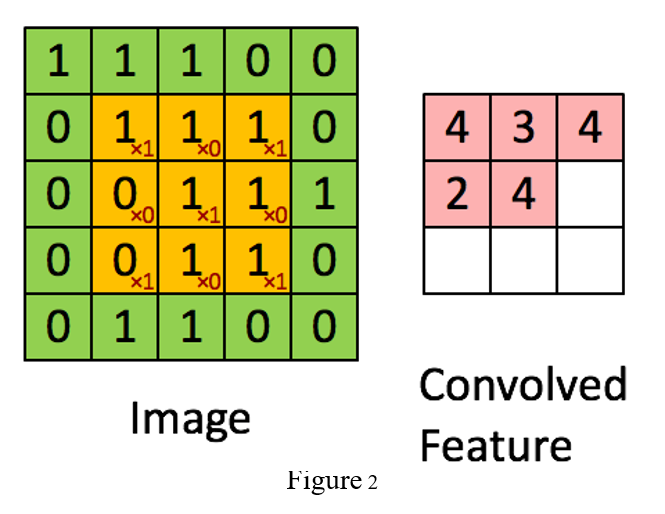

Neural Network

Neural Networks receive an input, and transform it through a series of hidden layers as shown in Figure 3. Each hidden layer is made up of a set of neurons, where each neuron is fully connected to all neurons in the previous layer. The last fully-connected layer is called the “output layer” and in classification settings it represents the class scores.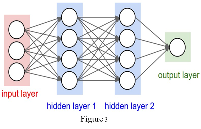

Convolution Neural Network

Simple CNN is a sequence of layers, and every layer of a CNN transforms one volume of activations to another through a differentiable function.

CNN LAYERS

• Input Layer - It is an input data like INPUT [$32\times 32 \times 3$] that will hold the raw pixel values of the image, in this case an image of width $32$, height $32$, and with three color channels R,G,B.
• Convolution Layer - It will compute the output of neurons that are connected to local regions in the input, each computing a dot product between their weights and a small region they are connected to in the input volume. This may result in volume such as [$32 \times 32 \times 12$] if we decided to use $12$ filters.
• Activation layer - It will apply an elementwise activation function, such as the $max(0,x)$ thresholding at zero. This leaves the size of the volume unchanged ([$32 \times 32 \times 12$]).
• Pooling Layer - It will perform a down sampling operation along the spatial dimensions (width, height), resulting in volume such as [$16 \times 16 \times 12$].
• Fully Connected Layer- FC (i.e. fully-connected) layer will compute the class scores, resulting in output layer. volume of size [$1 \times 1 \times 10$], where each of the $10$ numbers correspond to a class score.
• Output Layer – It contains score for each class such as volume of size [$1 \times 1 \times 10$], where each of the $10$ numbers correspond to a class score.

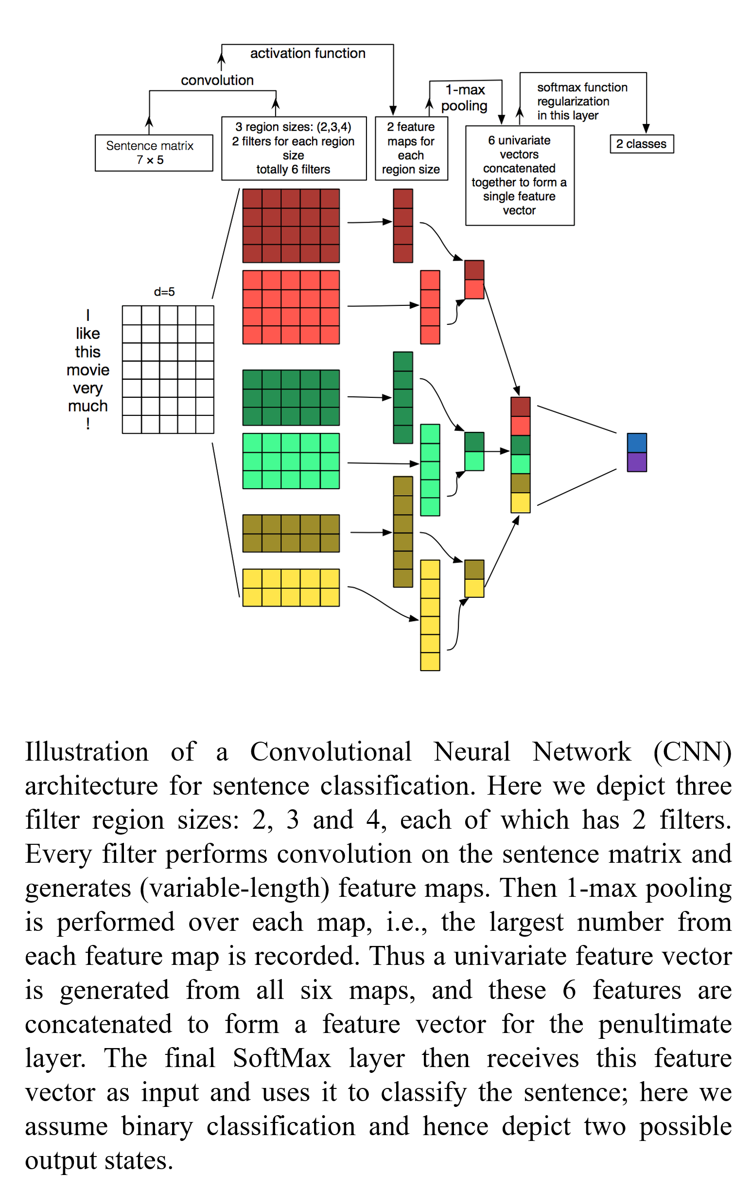
METHOD

• Word Vector : $x_i \in R^k$
• Sentence : $x_{1:n} = x_1 \oplus x_2 \oplus ……. \oplus x_n$ (vector concatenated).
• Concatenation of the words in the range : $x_{i:i+j}$
• Convolutional filter : $w \in R^{hk}$( goes over windows of h words)
• h could be 2 or higher :
• Filter $w$ is applied to all possible windows of concatenated vectors.
• All possible windows of length h $: {x_{1:h}, x_{2:h+1}, ….. , x_{n - h + 1 : n}}$.
• Results is a features map $: c = [c_1, c_2, ……. , c_{n - h + 1}] \in R^{n - h + 1}$
• New building block : pooling
  • In particular max-over-time pooling layer. In general max pooling are applied to 2D feature plane like CNN computer vision task where as max pooling over time is applied to 1D feature vector like NLP.
  • Idea: captures most important activation (maximum over time).
  • From feature map $c \in R^{n - h + 1}$ pooled single number: $\hat{c} = max {c}$
  • Since we want more features use maximum filter weights $w$.
  • It is useful to have different window sizes $h$.