
Topological Complexity of Robot Motion Planning
Published:
Introduction
Topology is usually discussed in robotics through the notion of configuration spaces. For any mechanical system $R$, configuration space is the variety of all possible states ($X$). In general, $X$ is determined by real parameters which can be stated as a subset of Euclidian space($\mathbb{R}^k$ )
Examples:
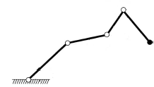
- Robot Arm; Latombe, 1991. Robot arm consists of $4$ bars with endpoints as revolving joints as shown in Figure 1. If the bar is only allowed motion in a $2$ dimensional plane. Then each bar is allowed to move in a circle ($S^1$) independently and its configuration space is $X = S^1 \times S^1 \times S^1 \times S^1$ i.e a $4$-dimensional torus. If each bar is allowed motion in $3$ dimension then its configuration space is $X = S^2 \times S^2 \times S^2 \times S^2$. Note: self-intersection of the arm is allowed.
- Let $W$ is a topological space and $X = F(W, n)$ denote Cartesian product $W \times …… \times W$, $n$ times contains tuple $(w_1,….., w_n)$ such that $w_i \neq w_j$ whenever $i \neq j$. $X = F(W, n)$ is usual configuration space for collision free motion of $n$ particles.
 |
|---|
| Figure 1 |
Motion Planning Algorithm
For a given mechanical system $R$ motion planning algorithm is a function that assigns to each ordered pair $(A, B)$ where $A$ is the initial state and $B$ is a final state a continuous motion of the mechanical system which starts at $A$ and ends at $B$. Let $X$ is the configuration space of the mechanical system and states are represented by points in $X$. Continuous motion of the system from state $A$ to $B$ is represented by continuous path $\gamma: [0, 1] \to X$, where $\gamma(0)= A$ and $\gamma(1)= B$. The system is path-connected if there exists a $\gamma$ for any arbitrary $A$ and $B$.
$PX = X^I$ is the space of all continuous paths $\gamma: I=[0, 1] \to X $ $PX$ is supplied with compact open topology (compact-open topology is a topology defined on the set of continuous maps between two topological spaces). For any space $Y$ let $p: Y^I \to Y \times Y$ be the map $p(\gamma) = (\gamma(0), \gamma(1))$ for $\gamma: I\to Y$. Then $p$ is fibration. Let $\pi : PX \to X \times X$ is a map where any path $\gamma \in PX$ is mapped to $(\gamma(0), \gamma(1)) \in X\times X$. Then $\pi$ is a fibration.
Definition 2.1
The motion planning algorithm 1 is a section of a fibration. Let $s$ motion planning algorithm i.e a map $s: X \times X \to PX$ where $\pi \circ s = 1_{X \times X}$. Note $ s(A, B) = \gamma \in PX $ where $\gamma $ is a continuous function of $t \in I$ for given points $A, B \in X$. And $s$ is continuous, if suggested route($s(A, B)$) depends continuously on states $A$ and $B$. Under what condition $s$ is continuous?. We will talk about it before that few definitions.
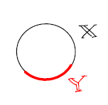
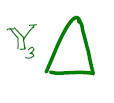
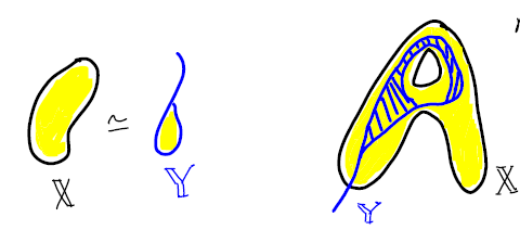
Let $f, g: X \to Y$ be continuous maps from topological space $X$ to space $Y$. A homotopy between $f$ and $g$ is another continuous map, $H : X \times [0, 1] \to Y$ such that $H(x, 0) = f(x)$ and $H(x, 1) = g(x) \forall x \in X$, i.e., $f \simeq g$. Equivalence relation implies reflexive, symmetric, transitive. Now we extend definition of homotopy to topological spaces.$Y \subseteq X$ is a retract of $X$ if there is a continuous map $r: X \to Y$ with $r(y) = y ~~\forall y \in Y$, then $r$ is a retraction. An example is shown in Figure 2.a .$Y$ is a deformation retract of $X$ and $r$ is deformation retraction, if there is a homotopy between the retract $r$ and the identity map ${id}_{X}$ on $X$ i.e \(r \simeq {id}_{X}\). Deformation retraction implies homotopy equivalence between topological space $X \simeq Y$. Some examples are shown in Figure 2. $X$ and $Y$ homotopy equivalent or have the same homotopy type, if there exists continuous maps $f: X \to Y$ and $g: Y \to X$ such that \(f \circ g \simeq {id}_{Y}\) and \(g \circ f \simeq {id}_{X}\). Denoted by $X \simeq Y$. Some examples are shown in Figure 3.
 |
|---|
| Figure 2.a |
 |
| Figure 2.b |
 |
| Figure 2.c |
 |
| Figure 2.d |
| Figure 2 : $Y$ is not a deformation retraction of $X$ but just a retraction, whereas $Y_i$ $\forall i \in {1, 2, 3, 4}$ is deformation retraction of $X$. Hence \(X \simeq Y_i ~~\forall i\) 2 |
 |
|---|
| Figure 3: $X \simeq Y$(homotopy equivalent) but $Y$ is not a retract of $X$ in the figure on right implies deformation retract is not a necessary condition for homotopy equivalence. 2 |
Definition 2.2
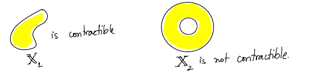
If $Y$ is a single point and $X \simeq Y$, then $X$ is contractible. Some examples are shown in figure 4.2
 |
|---|
| Figure 4 |
Lemma 2.3
A continuous motion planning algorithm in $X$ exists if and only if space $X$ is contractible. For a system with a non-contractible configuration space, any motion planning algorithm must be discontinuous .1
Topological Complexity TC(X)
Polyhedral is a subset $X \subset \mathbb{R}^n$, homeomorphic to underline space of some finite-dimensional simplicial complex.
Definition 3.1
Let $X$ be a polyhedron. A motion planning algorithm $s: X \times X \to PX$ is called tame if $X \times X$ can be split into finitely many sets 1 $ X \times X = F_1 \cup F_2 \cup ….. \cup F_k $ such that
- The restriction \(s \mid F_i : F_i \to PX\) is continuous, $i \in \{1, ….. , k\}$
- $F_i \cap F_j = \emptyset$, where $i \neq j$
- Each $F_i$ is a Euclidean Neighborhood Retract (ENR), defined below.
Let $A \subset X$. Then A is a neighborhood retract (in $X$), if $A$ has a neighborhood($N_A$) in $X$ and $N_A$ is a retract of $X$. Every retract is also a neighborhood retract but every neighborhood retract not necessarily a retract. For example: $X = [0 ,1]$ and $A = \{0\} \cup \{1\}$ then A is a neighborhood retract but not a retract. Since map $r$(retract) is not continuous. If $X = \mathbb{R}^n$, then $A$ is euclidean neighborhood retract 3.
The topological complexity of the tame motion planning algorithm($s$) is the minimum number of domains($k$) such that $s$ is continuous for each domain. Topological complexity ($TC(X)$) of finite-dimensional polyhedron $X$ is minimal topological complexity of tame motion planning algorithms in $X$.1
Some of the topological complexity $TC(X)$ examples:
If X is contractible then by lemma 2.3 there exists a continuous tame motion planning algorithm. Hence $TC(X) = 1$. Given topological space $X = S^n$, where $n$ is odd. Consider $F_1 = \{(A, B)\mid A \neq -B\}$. Then $s_1: F_1 \to PX$ where $s_1(A, B)$ is a shortest geodesic arc along the surface of $S^n$. Consider $F_2 = \{(A, -A)\}$ i.e pair of all antipodal points. We will find $s_2: F_2 \to PX$. Construct non vanishing vector field $v$ on $S^n$. Then $s_2(A, -A)$ move along the semi circle tangent to vector $v(A)$ from $A$ to $-A$ . And $X \times X = F_1 \cup F_2$, $TC(X) = 2$. Note: $v$ is non vanishing since n is odd.
Given topological space $X = S^n$, where $n$ is even. Since $n$ is even any vector field $v$ has at least one zero. We may construct a vector field $v$ with one zero at $A_0$ i.e $v(A_0) = 0$. Then $F_1$ remains same as in second and $F_2 = \{(A, -A) \mid A \neq A_0\}$. Consider $F_3 = \{(A_0, -A_0)\}$ and $s_3: F_3 \to PX$ is defined by an arbitrary path from $A_0$ to $-A_0$. And $X \times X = F_1 \cup F_2 \cup F_3$, $TC(X) = 3$. Note: $v$ has one zero since n is even based on Hairy Ball Theorem.
Topological complexity is Homotopy invariant.
Lemma 3.2
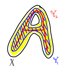
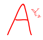
Let $X$ and $Y$ be topological spaces. Suppose that $X$ dominates $Y$ i.e there exist continuous maps $f: X \to Y$ and $g: Y \to X$ such that $f \circ g \sim {id}_Y$. Then $TC(Y) \leq TC(X)$.4 An example is shown in figure 5.
 |
| Figure 5.a |
 |
| Figure 5.b |
 |
| Figure 5.c |
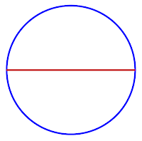
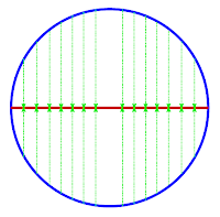
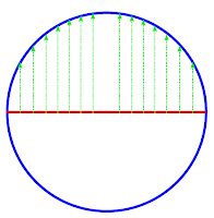
| Figure 5: $X$(unit circle) and $Y$(straight line) are topological space in blue and red. $f$ is a continuous map that projects every point of $X$ vertically on $Y$ as shown by green edges in middle figure. $g$ is continuous map that projects every points of $Y$ vertically onto upper semi circle $X$ as shown by green edges in right most figure. Then $f \circ g \sim {id}_Y$ i.e $X$ dominates $Y$ and $TC(X) =2$, $TC(Y) = 1$.|
Lemma 3.3
If $ Y \subset X$ is a retract. Then $TC(Y) \leq TC(X)$.1 Consider Figure 2.a, where $X$ is a unit circle and $Y$ is an arc smaller than half of the unit circle circumference. Based on example 2 of topological complexity $X \times X = F_1 \cup F_2$ since $X$ has antipodal points. But $Y$ has no antipodal points, hence $Y \times Y = F_1$. Hence $TC(Y) = 1$ and $TC(X) =2$.
Corollary 3.4
If $ Y \subset X$ is a retract and $X$ can be deformed into $Y$. Then $TC(Y) = TC(X)$. It is also true, if topological space $X$ and $Y$ are homotopy equivalent then $TC(X) = TC(Y)$[Mi2014]. Consider a topological space $Y$ homeomorphic to sphere($S^2$). That implies $Y$ is homotopy equivalent to $S^2$. Hence $TC(S^2) = TC(Y)$.
Relative Topological Complexity (\(TC_X(A)\))
Definition 4.1
Let $X$ be a topological space and $A \subset X \times X$ be subspace. Then the number \({TC}_{X}(A)\) is defined as the fibration \(\pi: P_{A}X \to A\) where \({P_A}X \subset PX\) is the space of all paths \(\gamma : [0, 1] \to X\) such that the pair if end points \((\gamma(0), \gamma(1))\) lies in $A$. In other words ${TC}_X(A)$ is the smallest integer $k$ such that there is an open cover $A = U_1 \cup ………… \cup U_k$ where $U_i \subset A$ is open and projections $g: U_i \to X, \tilde{g}: U_i \to \tilde{X}$ are homotopic where $\tilde{X} = X, A\subset X \times \tilde{X}$.[3]
We can clearly see that $TC(X) = {TC}_{X}(X \times X)$
If $A_1, …. , A_k \subset X \times X$ are open covers covering $X \times X$, then \(TC(X) \leq TC_X(A_1)+ ....... + TC_X(A_k)\)
Lemma 4.2
For a subset $A \subset X \times X$ the following properties are equivalent 1:
- ${TC}_X (A) = 1$.
- Projections $g: A \to X, \tilde{g}: A \to \tilde{X}$ are homotopic where $\tilde{X} = X, A\subset X \times \tilde{X}$. (It is true by definition 4.1)
- The inclusion $A \to X \times X$ is homotopic to a map $A \to X \times X$ with values in the diagonal $\Delta_{X} \subset X \times X$.
Navigation Function
Before we start talking about navigation functions we will define few things from differential geometry. For a real valued smooth function $f: M \to \mathbb{R}$ on a differentiable manifold $M$, the points where the differential of $f$ (${df}_p : T_p(M) \to \mathbb{R}$) vanishes are called critical points of $f$ and their images under $f$ are called critical values. $\Delta_p(f) $ is the gradient vector field determined by $f$. Given the Riemannian metric $<. , .>$, ${df}_p(v)$ is determined by the property that
\(<\Delta_p(f), v> = {df}_p(v)\),
\[{df}_p(v) = \sum_{i =1}^{n} v_i\frac{\partial f}{\partial {x_i}}\]If at a critical point $p$, the matrix of second partial derivatives( Hessian Matrix $H_pf$) is nonsingular, then $p$ is called a non-degenerate critical point; if the Hessian is singular then $p$ is a degenerate critical point. A smooth real-valued function on manifold $M$ is a Morse function if it has no degenerate critical points. For the functions from $\mathbb{R} \to \mathbb{R}$, f has a critical point at the origin if $b = 0$, which is non-degenerate if $c \neq 0$ (i.e $f$ is of the form $a + cx^2+ …$) and degenerate if $c = 0$ (i.e $f$ is of the form $a + dx^3+ ….$)5. Morse functions necessarily have isolated critical points.
Let critical points set is $S$ of smooth function $f: M \to \mathbb{R}$. If each point in $S$ belongs to some non-degenerate connected submanifold then $f$ is a Morse-Bott function.
Definition 5.1
Navigation Function 1: A smooth function $F: M \times M \to \mathbb{R}$ is called a navigation function for $M$ if
- $F(x, y) \geq 0$ for all $x, y \in M$
- $F(x, y) = 0$ if and only if $x = y$
- $F$ is nondegenerate in the sense of Morse-Bott function.
Set of critical points of $F$ belongs to a set of connected components ${S_i}$, where $S_i$ is submanifold and $ S_i \subset M \times M$. We are also assuming that that $S_1 = \Delta_{M}$, where $\Delta_{M} = {(x, x); x \in M }$.
Gradient vector Field ($\Delta_p F$) of $F$ at point $p$ is
\[\Delta_p F = \sum_{i =1}^{k} \frac{\partial F}{\partial x_i} e_i + \sum_{i =1}^{k} \frac{\partial F}{\partial y_i} e_{i + k}\]where \(p=(x^*_1, ...... , x^*_k, y^*_1, ......, y^*_k)= (x^*, y^*)\), \(v_{x^*} \in T_{x^*}(M), v_{y^*} \in T_{y^*}(M)\) and \((v_{x^*}, v_{y^*}) \in T_p(M \times M)\)
\[\sum_{i =1}^{k} \frac{\partial F}{\partial x_i} {v}^i_{x^*} + \sum_{i =1}^{k} \frac{\partial F}{\partial y_i} {v}^i_{y^*} = dF_p(v)\]where \(v=({v}_{x^*}, {v}_{y^*})\)
Lemma 5.2
Let $F: M \times M \to \mathbb{R}$ be a navigation function for $M$. Consider the connected components $S_1, S_2, ….., S_k \subset M \times M$ of the set of critical points of $F$ and denote by $c_i \in \mathbb{R}$ the corresponding critical values, i.e, $F(S_i) = {c_i}$ 1. Then one has \(TC(M) \leq \sum_{r \in Crit(F)} N_r\).Here $Crit(F) \subset \mathbb{R}$ denotes the set of critical values of $F$ and for $r \in Crit(F)$ the symbol $N_r$ denotes the maximum of the numbers ${TC}_M(S_i)$ where $i$ runs over indices satisfying $c_i = r$ i.e \(N_r = \max_{c_i =r} {TC}_M(S_i)\) Imagine, image of $F$ for some $S_i$ is the height $r$. $N_r$ is maximum relative topological complexity of all possible $S_i$ at a given height $r$. Topological complexity $M$ is less than or equal to the sum of $N_r$’s at all possible heights.
Example: Consider a navigation function $F : M \times M \to \mathbb{R}$ , where $M = S^1\times …… \times S^1 = T^n$ ($n$- dimensional torus) is given by \(F(x, y) = \sum_{i=1}^{k}(x_i - y_i)^2\) \(dF_p(v) = \sum_{i =1}^{k} 2(x^*_i - y^*_i) {v}^i_{x^*} - \sum_{i =1}^{k} 2(x^*_i - y^*_i) {v}^i_{y^*} = \sum_{i =1}^{k} 2(x^*_i - y^*_i) ({v}^i_{x^*} - {v}^i_{y^*}) ~~ (1)\)
Then, for \(dF_p(v) = 0\) i.e \(p=(x^*, y^*)\) is a critical point. It is true if and only if euclidean segment \((x^*, y^*) \subset R^n\) are perpendicular to tangent space to $M$ at point \(x^*\)(i.e \(T_{x^*}(M)\)) and \(y^*\) (i.e \(T_{y^*}(M)\)). It is clear from \(dF_p(v)\) equation 1. $x = (x_1, ……. , x_n) \in M, y = (y_1, ……… , y_n) \in M$ and $(x_i, y_i) \in M_i$, where $M_i$ is the $i^{th}$ $S^1$ in configuration space of $M$. Let $J \subseteq {1, …..,n}$ and $S_J$ is critical set of $M$, where $x_i = -y_i \forall i \in J$ and $x_i = y_i \forall i \notin J$ by equation 1. Let $J = {1, 2}$, then $F(S_J) = 4x^2_1+ 4x^2_2 = 4 \times 2 = 8$, since $x_1, x_2$ lies on a unit circle $S^1$ implies $x^2_1 = 1$ and $x^2_2 = 1$. We can clearly see that $F(S_J) = 4|J|$. Hence critical values $Crit(F) = {0, 4, 8, …….., 4n}$ and number of critical values are $n + 1$. We can clearly see that first and second projections $g, \tilde{g}$ of $S_J \to M$ are homotopic, hence $TC_M(S_J) = 1$ based on lemma 4.2. This implies that $N_r = 1$ for any $r\in Crit(F)$, hence by lemma 5.2 $TC(M) \leq n+1$.
References
Michael Farber, 2014. Invitation to topological robotics. ↩ ↩2 ↩3 ↩4 ↩5 ↩6 ↩7 ↩8
Bala Krishnamoorthy, 2018. Computational topology. http://www.math.wsu.edu/math/faculty/bkrishna/FilesMath574/S18/LecNotes/Lec9_Math574_02062018.pdf ↩ ↩2 ↩3
A. Dold., 1995. Lectures on Algebraic Topology. Classics in Mathematics. Springer Berlin Heidelberg, 1995. ↩
Michael Farber, 2017. Configuration spaces and robot motion planning algorithms (Lecture Notes). ↩
Wikipedia contributors, accessed 8-December-2019. Morse theory — Wikipedia, the free encyclopedia. https://en.wikipedia.org/w/index.php?title=Morse_theory&oldid=925851127 ↩